Ackley Function

April 29, 2022 - Reading time: 2 minutes

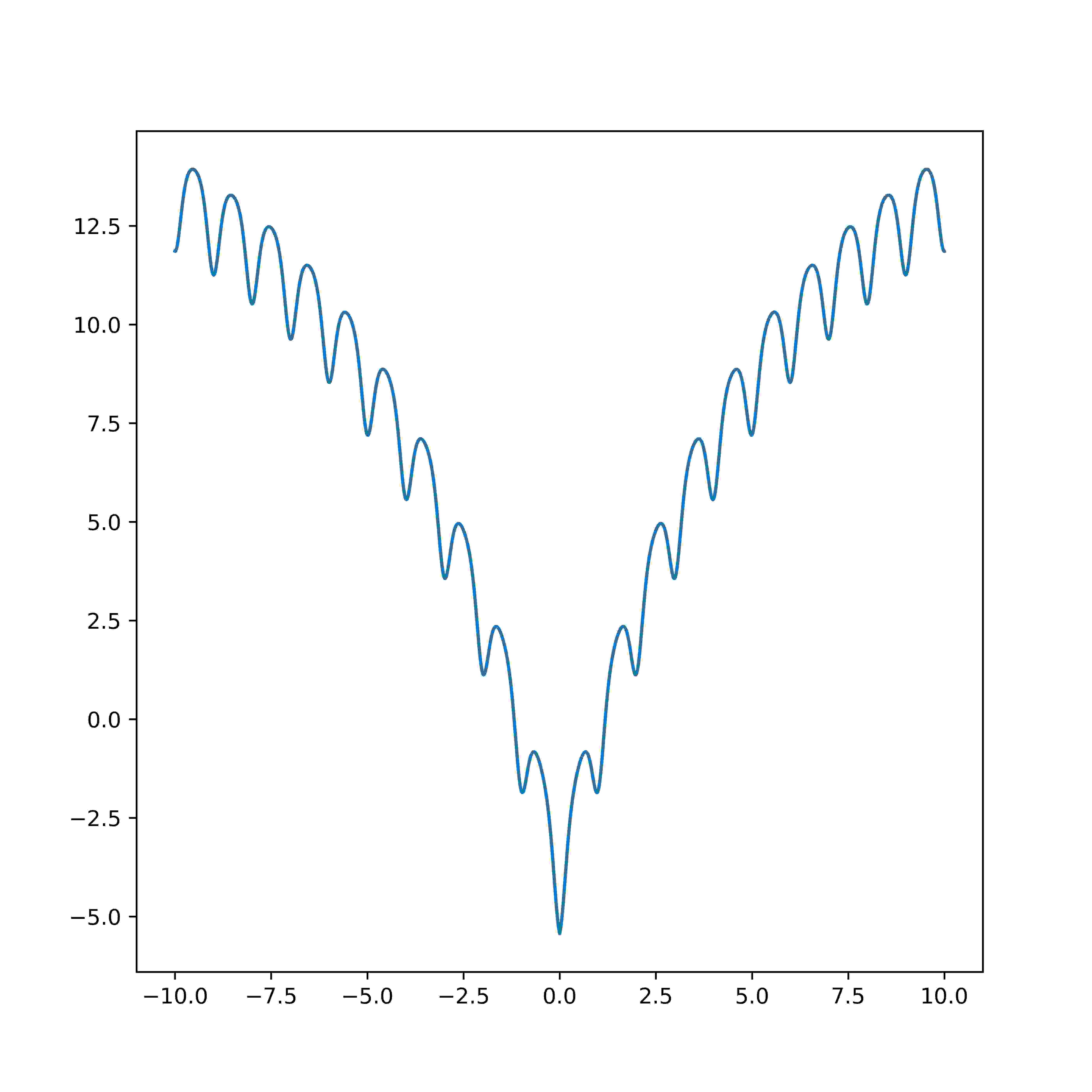
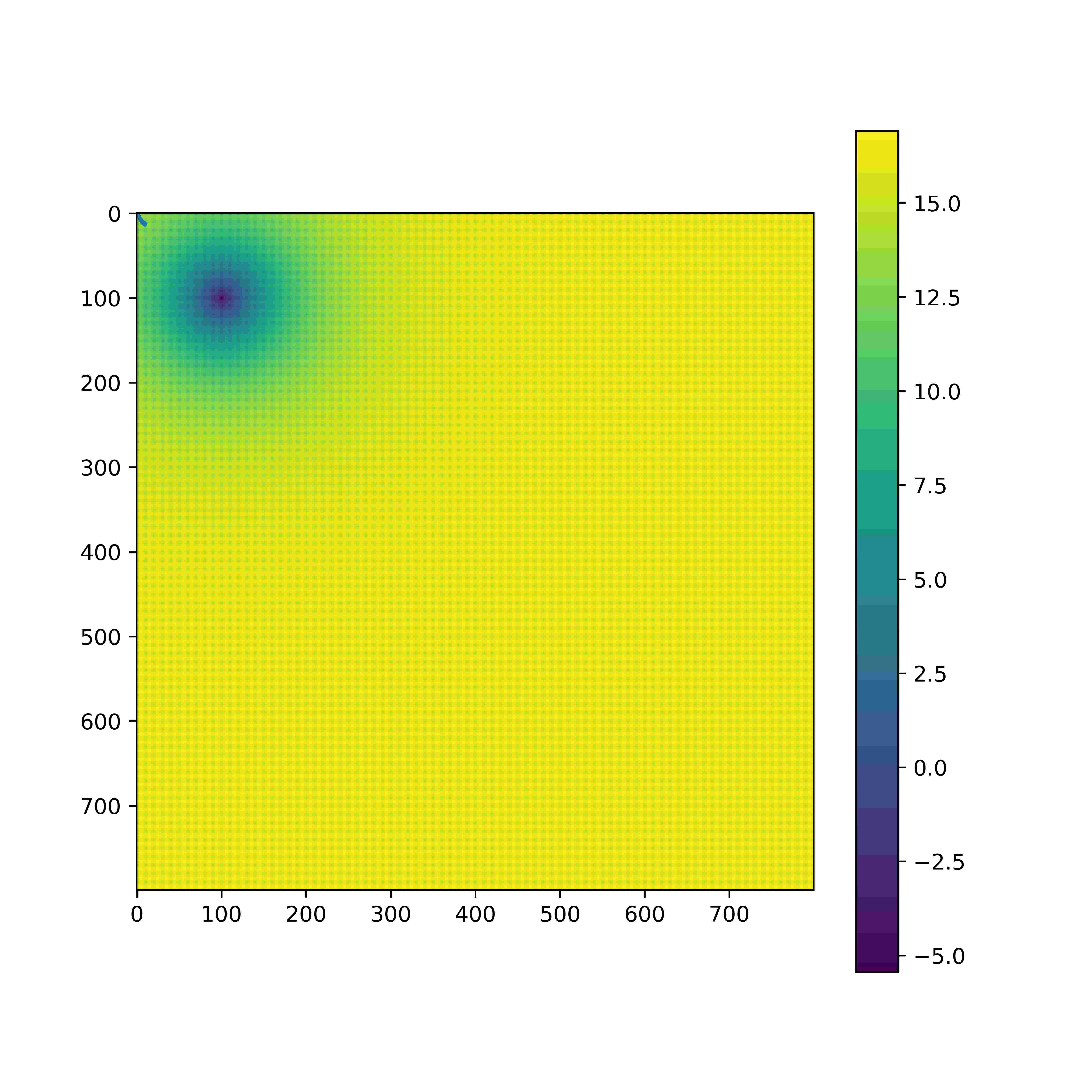
The Ackley function is widely used for testing optimization algorithms. In its two-dimensional form, as shown in the plot above, it is characterized by a nearly flat outer region, and a large hole at the centre. The function poses a risk for optimization algorithms, particularly hillclimbing algorithms, to be trapped in one of its many local minima.

Recommended variable values are: a = 20, b = 0.2 and c = 2π.

So,

import os
import matplotlib.pyplot as plt
import numpy as np
import math
import numba

plt.rcParams["figure.dpi"] = 150
plt.rcParams["figure.figsize"] = (7, 7)

SHOW = False
SAVE = True

def make_ackley(dimensions, a=20, b=0.2, c=2 * math.pi):
        @numba.jit
        def inner(*args):
                assert len(args) == dimensions
                x = 0
                for d in args:
                        x += d**2
                x *= 1 / dimensions
                x = math.sqrt(x)
                x *= -b
                result = -a * math.exp(x)

                x = 0
                for d in args:
                        x += math.cos(d * c)
                x *= 1 / dimensions
                result -= math.exp(x)

                result += a
                result -= math.exp(1)

                return result

        return inner

ackley_1d = make_ackley(1)

graph = [ackley_1d(x) for x in np.arange(-10, 10, 0.001)]

plt.plot(np.arange(-10, 10, 0.001), graph)

if SHOW:
    plt.show()
if SAVE:
    plt.savefig(os.path.join(os.path.dirname(__file__), "ackley2d.png"))

Out [1]: 

ackley_2d = make_ackley(2)

RES = 10
graph = np.zeros((80 * RES, 80 * RES))

for x in range(80 * RES):
    for y in range(80 * RES):
        graph[y][x] = ackley_2d((x / RES) - 10, (y / RES) - 10)

plt.imshow(graph)
plt.colorbar()

if SHOW:
    plt.show()
if SAVE:
    plt.savefig(os.path.join(os.path.dirname(__file__), "ackleyCmap.png"))

Out [2]: 

ackley_2d = make_ackley(2)

gx = []
gy = []
gz = []

for x in np.arange(-10, 10, 0.5):
    for y in np.arange(-10, 10, 0.5):
        gx.append(x)
        gy.append(y)
        gz.append(ackley_2d(x, y))

fig = plt.figure()
ax = fig.add_subplot(projection="3d")
_ = ax.plot_trisurf(gx, gy, gz)

if SHOW:
    plt.show()
if SAVE:
    plt.savefig(os.path.join(os.path.dirname(__file__), "ackley3d.png"))

Out [3]: